Intuitive Machine Learning

With all the hype around Machine Learning (ML) in modelling geology these days, it feels a bit like we are trying to jump the ML wagon too. In some ways, I guess that is true. But not because we like the hype so much. In this article we will share some results before going into a bit more details. That way you can quickly decide if you want to continue reading.

However, before we go on explaining our use of Machine Learning, let us make a distinction between AI (Artificial Intelligence) and Machine Learning (ML). As the name AI implies, it contains some intelligence specifically in decision making. In contrast, to us ML is about learning correlations within the data provided. There is no ‘intelligence’, that is left to the user.

Main idea

The main adoption that we made is in applying ML techniques for geological categorical data as opposed to numeric data like assays etc. The general aim of modelling geology is to reconstruct a 3D representation of the real 3D world from the limited data we have. We do this by labelling an area with certain categories like lithology. Those labels can be used for a classification system.  One of the major strengths of ML is that it is fast at classification, and that is essentially what modelling geology is all about: a point in 3D space is classified as being part of a unit, or not. Once we started approaching geological modelling as a set of classification functions we were quickly able to build realistic models using these ML classifiers.

In using ML techniques this way, they become very similar to the implicit modelling introduced to the industry over 2 decades ago. More about this can be found in our blog post Machine Learning Demystified.

A simple example

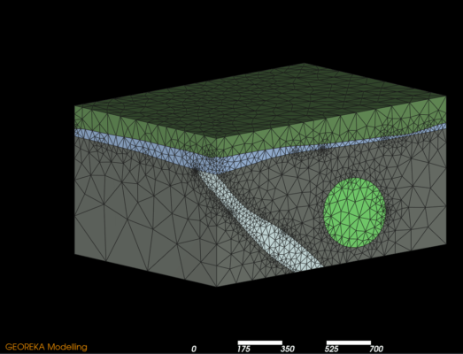
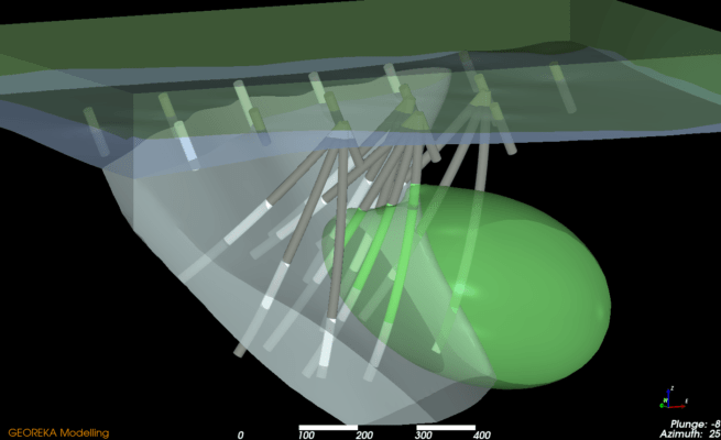
Let us look at a, to some, famous example: Marvin. It is a simple artificial data set. It has an Oxide layer (blue) on the top bounded by the topography, a Quartz porphyry (QzP) vein constrained below it and finally Granodiorite sitting against the QzP.

For each domain a function is created that defines the volume of that domain. Each domain can, and typically will, have its own anisotropy. Integrating the anisotropy with ML is no different than for implicit modelling.

Example geological modelling workflow

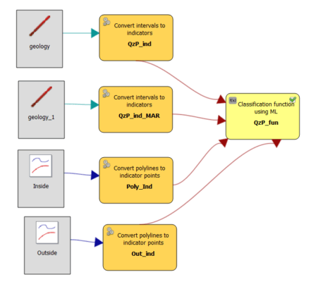
This model is created using ML techniques instead of implicit modelling. On the left we show an example workflow for modelling the QzP  domain from four different data sets: 2 exploration drill sets and 2 manually added control sets. The yellow box on the right contains the tool to train an ML classifier.

The only difference in this workflow compared to implicit modelling is that instead of interpolating numeric values (indicator points or distance values), we created a ML classifier for this domain. This means that all points belonging to a category, QzP in this instance, are labelled as inside (or +1 for historical perspective). All others are labelled as outside (or -1) before the ML classifier tries to separate the two groups.

Intuitive integration

To transition from established workflows to new ones like using ML tools it is always easiest to compare with what you already know. That is how we integrated ML into our modelling. In practise, this means we convert the unit to model into indicator values. This allows us to either use Ordinary Kriging, implicit modelling using RBF’s or the ML classifiers to ‘interpolate’ the data. In turn, this means the different methods and their results can be easily compared. To the user the workflows are identical except for the interpolation method used. Moreover, in our article Machine Learning demystified, we explain the similarities between ML and existing methods.

Download a 30 day free trial now Trial and Pricing