3D Geological Modelling
GEOREKA’s 3D geological modelling software is versatile and adaptable. It is a like a Swiss army knife with many different tools. In combination with its unique modelling approach it can be made to fit any project be it Mineral Exploration or Industrial Minerals. The heart of all modelling is a data-driven processing engine. This engine provides implicit, data-driven modelling tools for both geological and numerical features. Here we will provide quick overview of most fundamental tools.
Dynamic data-driven workflows
As mentioned above, the core of all geological modelling in GEOREKA is through its data-driven modelling engine. Compared to most other software, modelling is not a fixed process from input to output. Instead, a workflow needs to be developed that fits the problem at hand. Of course, many tasks will be similar between projects and these workflows can be re-used. However, GEOREKA provides the flexibility to adapt workflows even to the most unique problems.
Furthermore, the workflows are set up through a visible layout. This provides the added benefit that a single picture can explain a complete workflow.
To illustrate some examples.
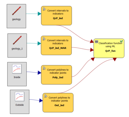
A workflow using multiple input data sets (2 drill sets, 2 manually added points) to create a domain function.
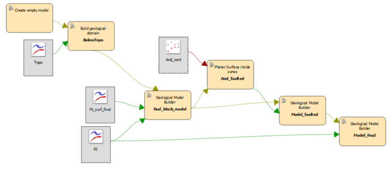
Traditional workflow demonstrating how two contacts can be used to define a geological domain.
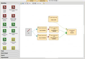
Another example of a traditional workflow where two contacts are used to define a domain. This time surfaces are not used directly. Instead, they are created from drill data and then applied a domain boundaries.
Domain functions
In GEOREKA version 4 a new concept was introduced. Instead of modelling geological units by their boundaries (contacts), functions are used to describe domains. But, not to worry, users do not need to do complex maths, that is what the software is for. By providing inside and outside points (those that either belong to the domain, or not), a function is estimated that describes the domain.
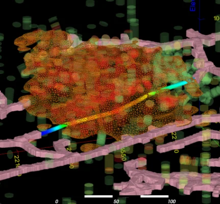
Functions can be created for geological domains like lithological. In the 3D display they appear as dynamic surfaces rendered using the latest from graphics developers (see our beyond conventional page).
Numeric interpolation
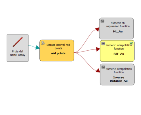
Similarly to modelling geology, numeric data can be interpolated using functions such as implicit (RBF), Ordinary Kriging or Inverse Distance, or the more modern Machine Learning regression. Each of those methods are also set up as a function that can either be used to define domains, or create numeric ‘block’ models.
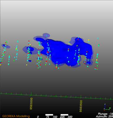
Again, a workflows needs to be set up first to create a functional representation of the interpolation method. Next, the function can be viewed in 3D with other data using real-time cut-offs, through the use of real-time raytracing. There they can be compared with other interpolation functions like we did here. The transparent blue ‘shell’ is the RBF interpolation function at 4 gr/t AU grades. The opaque blue is the result from Machine Learning regression also at 4 gr/t.
Once the correct settings have been found, the functions can be used to either evaluate them on a grid or an existing geological model, or they can be used directly within the model descriptor (see below).
Compare estimates and volumes
Compare estimation results from various interpolation methods like Inverse Distance Weighting, Radial Basis Functions (RBF) and Ordinary Kriging. To this end the interpolation functions will need to be evaluated on a grid such as a regular grid, or a prior built geological model. The information panel will then display the estimated average with the volume in the info panel.
Build models through descriptions
In GEOREKA models are not really built until they are needed. Building an actual model can be very time consuming and therefore is left as a specific step within the modelling process. To this end the user specifies all the domains and their relationships, specifically their relative ages, in a descriptor. This descriptor is like a list of steps the software needs to go through to build the complete model. At this stage, the relation between faults (which units are affected or not) and other domains are defined. The main rule is that a domain cannot overwrite another domain unless explicitly told to do so. In other words if unit A is already defined, unit B cannot intrude it. If that were needed, unit B (being younger) would need to be listed first, followed by unit A. As an example below is a descriptor for a stratigraphic model. Further examples can be found on our technical articles page.
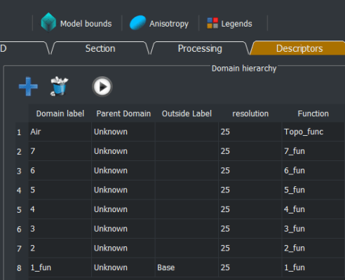
The model descriptor on the left lists all the domains that make up the model. The very first row uses the topography to remove all data above that topographic surfaces (labelled as air). In this example each subsequent domain is a stratigraphic layer. The youngest unit, 7 is the first in the list, the oldest unit 1, is the last.
The result is shown below, where several layers are hidden to better highlight the model.
